Simple signals

We are ready to try swan on some really simple data series. First, let's construct the data. It will be a signal with two harmonic rhythms of identical amplitude at two different frequencies, say, at 1.2 and 3.7 Hz, discretized at 65 Hz of 16 sec in length. These parameters are, of course arbitrary and could be chosen any at you will.

The signal can be easily made in Pylab using the following commands:

Fs = 65.0
time  = arange(0,16,1/Fs)
signal = sin(2*pi*1.2*time) + cos(2*pi*3.7*time)
save('signal.dat', signal)

or in the Octave with the following commands:

Fs = 65.0;
time  = [0:1/Fs:16];
signal = sin(2*pi*1.2*time) + cos(2*pi*3.7*time);
save('-ascii', 'signal.dat', signal)

this should be the same in Matlab(tm), except for the data saving command.

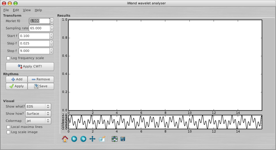
So, we can start swan, and in the 'File' menu select 'Open' and pick the signal.dat file. Then, we change the sampling frequency associated with the signal in the 'Sampling rate' field to the value 65 Hz. Alternatively, we can tell swan the sampling rate and the data file via command options, like that:

swan -s 65 signal.dat

The result we should obtain so far is shown in the figure (click to see the larger version):

Now change the 'Start f' to 0.5, this is the frequency we start from, 'Step f' to 0.2, this is the step in frequencies we use in the wavelet transform, and set 'Stop f' to 6.0 (guess what does it stand for). Click the 'Apply CWT!' button. The energy density surface (EDS) should appear as in the following figure:

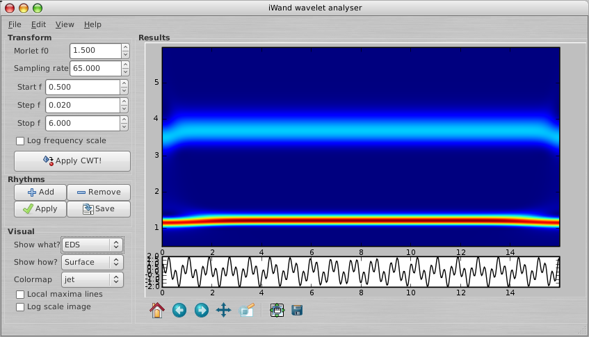
Basically, one could think of the EDS as a surface made of the instantaneous energy spectra of the signal. Indeed, we see two rhythms, one at 1.2 Hz, the other at 3.7 Hz. Note that on the edge of the signal the frequency of the rhythm is distorted, this just results from the finite signal length.

The rhythm at lower frequency is higher in amplitude (more red) and thinner in the frequency domain. The one at higher frequency is broader and lower in amplitude. This is inevitable with wavelet-based spectra and is related to the energy distribution in the wavelet. See what changes if you change the f0 of the Morlet wavelet and click the 'Apply CWT!' button again.

If you are interested in the rhythm amplitude, not in the energy, you can plot the results with amplitude correction (in general, EDS*f). In the 'Show what?' combo box select 'EDS-A' to obtain this. The result is shown in the following figure. I also changed the colormap, just to show that you can do that too:

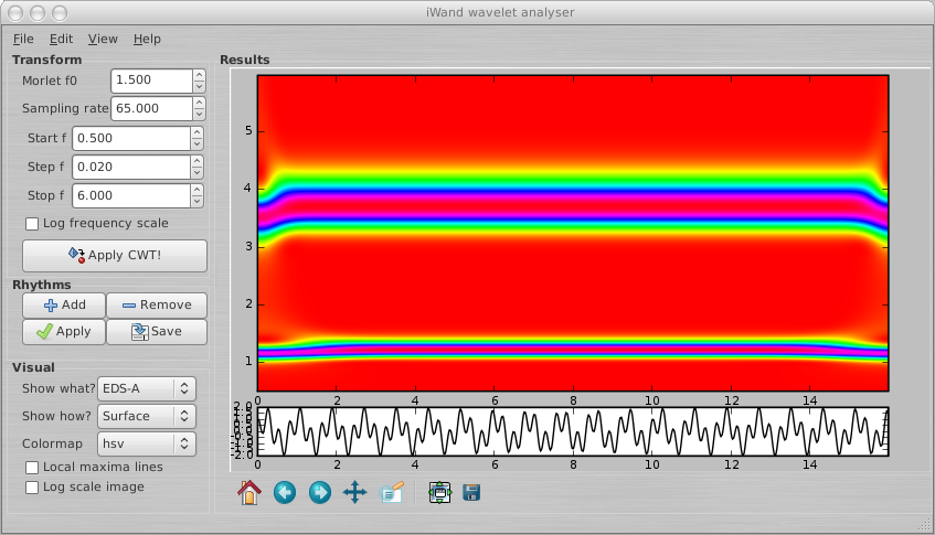
The broadness of the peaks didn't change, but the amplitudes are equal now.

By the way, in the tarball you will find a sample signal file with two frequencies, discretized at 62.5 Hz. See if you can find out which those frequencies are and how do they look like in swan.

If you check the 'Local maxima lines' check-box, you will see long yellow lines following the ridges of the two rhythms.